How To Find A Cdf From A Pdf

4.ane: Probability Density Functions (PDFs) and Cumulative Distribution Functions (CDFs) for Continuous Random Variables

Last updated
Save every bit PDF

Page ID: 3265

Probability Density Functions (PDFs)

Call up that continuous random variables accept uncountably many possible values (call up of intervals of real numbers). Just as for discrete random variables, we can talk virtually probabilities for continuous random variables using density functions.

Definition $\PageIndex{one}$

The probability density function (pdf), denoted $f$, of a continuous random variable $X$ satisfies the post-obit:

$f(x) \geq 0$, for all $x\in\mathbb{R}$
$f$ is piecewise continuous
$\displaystyle{\int\limits^{\infty}_{-\infty}\! f(x)\,dx = ane}$
$\displaystyle{P(a\leq 10\leq b) = \int\limits^a_b\! f(10)\,dx}$

The kickoff three atmospheric condition in the definition country the properties necessary for a part to be a valid pdf for a continuous random variable. The 4th condition tells us how to use a pdf to calculate probabilities for continuous random variables, which are given pastintegrals the continuous analog to sums.

Case $\PageIndex{1}$

Permit the random variable $X$ denote the fourth dimension a person waits for an lift to arrive. Suppose the longest one would need to look for the lift is 2 minutes, and so that the possible values of $10$ (in minutes) are given by the interval $[0,ii]$. A possible pdf for $X$ is given by
$$f(x) = \left\{\begin{array}{l l}
x, & \text{for}\ 0\leq x\leq one \\
2-x, & \text{for}\ one< ten\leq 2 \\
0, & \text{otherwise}
\end{array}\correct.\notag$$
The graph of $f$ is given below, and we verify that $f$ satisfies the first 3 conditions in Definition 4.1.1:

From the graph, it is clear that $f(x) \geq 0$, for all $x \in \mathbb{R}$.
Since there are no holes, jumps, asymptotes, we come across that $f(x)$ is (piecewise) continuous.
Finally we compute:
$$\int\limits^{\infty}_{-\infty}\! f(x)\,dx = \int\limits^{2}_0\! x\,dx = \int\limits^1_0\! 10\,dx + \int\limits^2_0\! (ii-x)\,dx = 1\notag$$

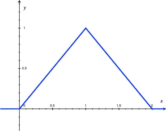
Figure 1: Graph of pdf for $10$, $f(x)$

So, if we wish to summate the probability that a person waits less than 30 seconds (or 0.five minutes) for the lift to arrive, then we calculate the post-obit probability using the pdf and the fourth property in Definition 4.1.ane:
$$P(0\leq 10\leq 0.v) = \int\limits^{0.5}_0\! f(x)\,dx = \int\limits^{0.five}_0\! x\,dx = 0.125\notag$$

Annotation that, unlike discrete random variables, continuous random variables accept null point probabilities , i.e., the probability that a continuous random variable equals a unmarried value is ever given by 0. Formally, this follows from backdrop of integrals:
$$P(X=a) = P(a\leq 10\leq a) = \int\limits^a_a\! f(x)\, dx = 0.\notag$$
Informally, if we realize that probability for a continuous random variable is given by areas under pdf's , then, since at that place is no area in a line, at that place is no probability assigned to a random variable taking on a single value. This does not mean that a continuous random variable will never equal a single value, but that we exercise non assign any probability to unmarried values for the random variable. For this reason, we only talk about the probability of a continuous random variable taking a value in an INTERVAL, not at a betoken. And whether or not the endpoints of the interval are included does not bear on the probability. In fact, the following probabilities are all equal:
$$P(a\leq 10\leq b) = P(a<Ten<b) = P(a\leq X< b) = P(a< X \leq b) = \int\limits^b_a\!f(x)\,dx\notag$$

Cumulative Distribution Functions (CDFs)

Recall Definition three.ii.ii, the definition of the cdf, which applies to both discrete and continuous random variables. For continuous random variables we tin further specify how to summate the cdf with a formula as follows. Let $X$ take pdf $f$, so the cdf $F$ is given by
$$F(x) = P(10\leq x) = \int\limits^x_{-\infty}\! f(t)\, dt, \quad\text{for}\ x\in\mathbb{R}.\notag$$
In other words, the cdf for a continuous random variable is plant by integrating the pdf. Annotation that the Fundamental Theorem of Calculus implies that the pdf of a continuous random variable tin be found by differentiating the cdf. This relationship betwixt the pdf and cdf for a continuous random variable is incredibly useful.

Relationship between PDF and CDF for a Continuous Random Variable

Let $X$ exist a continuous random variable with pdf $f$ and cdf $F$.

Past definition, the cdf is plant by integrating the pdf:
$$F(x) = \int\limits^x_{-\infty}\! f(t)\, dt\notag$$
Past the Fundamental Theorem of Calculus, the pdf can exist found by differentiating the cdf:
$$f(x) = \frac{d}{dx}\left[F(ten)\right]\notag$$

Case $\PageIndex{2}$

Continuing in the context of Example iv.1.1, nosotros find the corresponding cdf. Get-go, let'south observe the cdf at 2 possible values of $X$, $x=0.v$ and $x=1.5$:
\begin{align*}
F(0.five) &= \int\limits^{0.v}_{-\infty}\! f(t)\, dt = \int\limits^{0.5}_0\! t\, dt = \frac{t^ii}{2}\bigg|^{0.5}_0 = 0.125 \\
F(1.5) &= \int\limits^{ane.five}_{-\infty}\! f(t)\, dt = \int\limits^{1}_0\! t\, dt + \int\limits^{1.5}_1 (2-t)\, dt = \frac{t^2}{2}\bigg|^{i}_0 + \left(2t - \frac{t^two}{2}\right)\bigg|^{1.5}_1 = 0.5 + (1.875-i.five) = 0.875
\end{align*}
Now we observe $F(x)$ more than generally, working over the intervals that $f(ten)$ has different formulas:
\begin{align*}
\text{for}\ x<0: \quad F(x) &= \int\limits^x_{-\infty}\! 0\, dt = 0 \\
\text{for}\ 0\leq ten\leq 1: \quad F(10) &= \int\limits^{x}_{0}\! t\, dt = \frac{t^two}{2}\bigg|^x_0 = \frac{10^2}{two} \\
\text{for}\ 1<ten\leq2: \quad F(x) &= \int\limits^{1}_0\! t\, dt + \int\limits^{x}_1 (2-t)\, dt = \frac{t^2}{two}\bigg|^{1}_0 + \left(2t - \frac{t^two}{ii}\correct)\bigg|^x_1 = 0.v + \left(2x - \frac{x^ii}{2}\correct) - (2 - 0.5) = 2x - \frac{x^ii}{2} - 1 \\
\text{for}\ x>ii: \quad F(ten) &= \int\limits^x_{-\infty}\! f(t)\, dt = 1
\end{align*}
Putting this altogether, we write $F$ as a piecewise function and Figure 2 gives its graph:
$$F(x) = \left\{\begin{array}{50 l}
0, & \text{for}\ x<0 \\
\frac{ten^ii}{ii}, & \text{for}\ 0\leq x \leq i \\
2x - \frac{10^2}{2} - 1, & \text{for}\ 1< x\leq 2 \\
1, & \text{for}\ x>two
\stop{array}\right.\notag$$

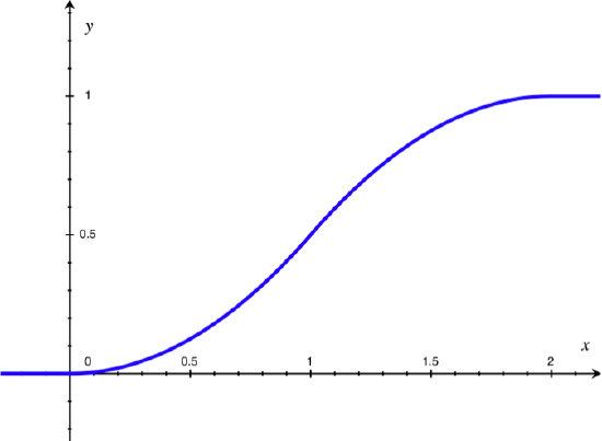
Screen Shot 2019-02-24 at 11.10.35 PM.png

Figure 2: Graph of cdf in Example 4.1.ii

Recall that the graph of the cdf for a discrete random variable is e'er a step function. Looking at Figure ii above, we note that the cdf for a continuous random variable is always a continuous function.

Percentiles of a Distribution

Definition $\PageIndex{two}$

The (100p)th percentile ($0\leq p\leq one$) of a probability distribution with cdf $F$ is the value $\pi_p$ such that $$F(\pi_p) = P(Ten\leq \pi_p) = p.\notag$$

To find the percentile $\pi_p$ of a continuous random variable, which is a possible value of the random variable, we are specifying a cumulative probability $p$ and solving the following equation for $\pi_p$:
$$\int^{\pi_p}_{-\infty} f(t)dt = p\notag$$

Special Cases: In that location are a few values of $p$ for which the corresponding percentile has a special name.

Median or $fifty^{th}$ percentile: $\pi_{.5} = \mu = Q_2$, separates probability (area under pdf) into two equal halves
1st Quartile or$25^{th}$ percentile: $\pi_{.25} = Q_1$, separates $1^{st}$ quarter (25%) of probability (expanse) from the rest
3rd Quartile or $75^{thursday}$ percentile: $\pi_{.75} = Q_3$, separates $3^{rd}$ quarter (75%) of probability (area) from the rest

Example $\PageIndex{three}$

Standing in the context of Example four.1.2, we find the median and quartiles.

median: find $\pi_{.v}$, such that $F(\pi_{.five}) = 0.5 \Rightarrow \pi_{.5} = 1$ (from graph in Effigy one)
1st quartile: find $Q_1 = \pi_{.25}$, such that $F(\pi_{.25}) = 0.25$. For this, nosotros use the formula and the graph of the cdf in Effigy 2:
$$\frac{\pi_{.25}^2}{2} = 0.25 \Rightarrow Q_1 = \pi_{.25} = \sqrt{0.five} \approx 0.707\notag$$
3rd quartile: find $Q_3 = \pi_{.75}$, such that $F(\pi_{.75}) = 0.75$. Again, use the graph of the cdf:
$$ii\pi_{.75} - \frac{\pi_{.75}^2}{two} - 1 = 0.75\ \Rightarrow\ (\text{using Quadratic Formula})\ Q_3 = \pi_{.75} = \frac{4-\sqrt{2}}{2} \approx 1.293\notag$$

Source: https://stats.libretexts.org/Courses/Saint_Mary's_College_Notre_Dame/MATH_345__-_Probability_(Kuter)/4%3A_Continuous_Random_Variables/4.1%3A_Probability_Density_Functions_(PDFs)_and_Cumulative_Distribution_Functions_(CDFs)_for_Continuous_Random_Variables

Posted by: schuleroulk1944.blogspot.com